Is My Data Normal?

Motivation

An HRV number in isolation means little. Is an SDNN of 74 ms high, low, or unremarkable? The honest answer is "compared to what?" This use case builds the missing reference frame: a normative prior fitted from large open normal-sinus-rhythm datasets, against which any new window can be scored as a quantile z-equivalent: a single, interpretable "how unusual is this?" number per feature.

Method

The normative reference is fitted once, from two PhysioNet normal-sinus-rhythm collections pooled together (nsrdb + nsr2db). Each recording is cut into 360-beat windows with a 120-beat stride, every window is scored through the 53-feature registry, and each feature's pooled distribution is fitted to an analytical family (Normal, Gamma, Beta, or LogNormal, chosen per feature). The result is 61 715 pooled healthy windows summarised as one fitted prior distribution per feature. The fitted priors ship in docs/normative_priors.csv; a few examples:

Given a fitted prior with CDF $F$ for a feature, a new value $x$ is scored as a quantile z-equivalent:

\[z = \Phi^{-1}\!\big(F(x)\big)\]

where $\Phi^{-1}$ is the standard-normal quantile function. This maps any distribution family onto a common $\sigma$-scale without assuming symmetry: a value at the prior's median scores $z = 0$, one at its 84th percentile scores $z \approx +1$. The same idea, applied to a user's own history instead of the population, gives the personal z-equivalent baseline_z used in the live tool.

Because the prior families are asymmetric where the biology is asymmetric, the dispersion bands drawn around each feature are distribution-aware central quantile intervals: the 68.27 % / 95.45 % / 99.73 % intervals standing in for ±1σ / ±2σ / ±3σ, rather than naive mean ± σ bands. The frequency-domain features default to a Welch periodogram on the resampled RR series (config["freq_method"] == :welch), with the raw unevenly-sampled Lomb–Scargle periodogram (Lomb, 1976), (Scargle, 1982) available as an alternative (config["freq_method"] = :lomb_scargle); the whole panel follows the standard HRV measurement conventions (Task Force, European Society of Cardiology / North American Society of Pacing & Electrophysiology, 1996).

Validity check: do the two healthy datasets agree?

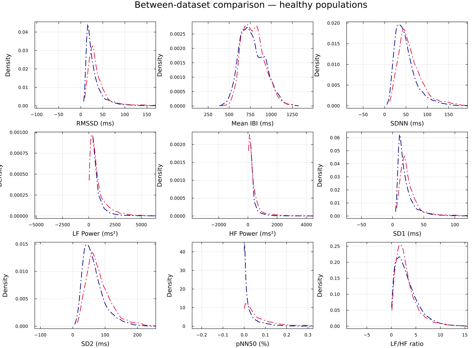
Before trusting a pooled prior, the two source datasets are compared directly. The between-dataset KDE overlay shows nsrdb and nsr2db tracing nearly the same feature distributions: evidence that "healthy" is a stable reference here and the pooling is legitimate.

Result: a live "how normal is this?" overlay

The scoring is wired into a real-time visualization. default_normative() draws the standard live HRV panels and overlays, on every panel, the personal-baseline percentile band (shaded low–high with a median line) plus, in each panel title, the current value's percentile and z-equivalent. So as beats stream in, each feature is continuously placed against the reference: the operational answer to "is my data normal, right now?"

The offline counterpart, plot_normative_kde_comparison, renders the same idea as a small-multiples grid: one KDE per feature, the fitted prior density overlaid as a dashed curve, and the σ-equivalent bands shaded behind it. The meditation use case shows this grid applied to a real cohort.

These priors are descriptive references from healthy cohorts, not clinical thresholds. A large $|z|$ means unusual relative to this reference population, not abnormal in any medical sense.

Build your own personal baseline

The personal-baseline band in default_normative() comes from a per-feature quantile grid (101 points, q0 to q100) computed over your own recording history. The artifact is not shipped with the package because it is personal data; you generate it once, locally, and the repository ignores the output path so it cannot be committed by accident.

You need a folder of your own IBI recordings as plain-text files, one inter-beat interval per line in milliseconds (the read_txt format), laid out as <EXPORT_DIR>/<PARTICIPANT>/*.txt. Then run:

PARTICIPANT=YourName EXPORT_DIR=path/to/your/exports \
  julia --project=. test/tools/generate_personal_baseline.jl

The tool preprocesses each recording (replace_zeros, replace_bio_outliers, interpolate_nans), cuts it into 100-beat windows with a 25-beat stride to match the live visualization, computes the windowed quantities, and writes the quantile grids to docs/personal_baseline_w100.csv, the default path default_normative() reads. WINDOW_SIZE, STRIDE, and OUTPUT can be overridden with environment variables; if you write to a custom location, pass it explicitly:

using HeartRateLab, GLMakie, LSL
HeartRateLab.Visualization.default_normative(; baseline="path/to/my_baseline.csv")

More recordings make a better baseline: the band is only as representative as the history behind it. Without a baseline file, default_normative() stops with a message pointing here, and the plain default() visualization works with no setup.

Reproduce / where the data lives

• Fitted priors: docs/normative_priors.csv (family, parameters, KS p-value, and n per feature; datasets = nsrdb+nsr2db, window_size = 360, stride = 120).
• Scoring API: HeartRateLab.Features.normative_prior(name) returns the fitted Distribution; the quantile z-equivalent is Φ⁻¹(cdf(prior, x)).
• Live overlay: HeartRateLab.Visualization.default_normative(; low=10, high=90) (needs GLMakie + an LSL RR stream; personal-baseline artifact built as described above).
• Offline plot: HeartRateLab.Visualization.plot_normative_kde_comparison.
• Dataset collection: test/tools/collect_normative_datasets.jl.

See the Visualization page for the full plotting API and the HRV Variable Zoo for each feature's normative distribution in detail.